
Fasanara Smart Fintech.
Investing in a
Digital Future.
Fasanara Smart Fintech.
Investing in a
Digital Future.
Weekly Performance
Another positive week for the S&P500 futures, with a 2.04% gains (vs + 3.30% lest week). Average trading volume was 1,266,00 contracts, 3.5% lower than last week.


Insights

Figure 4: S&P500 daily closing price between 2000 and 2020 with an overlay of the ETAS and Ricci Curvature-based indicators in Fasanara’s toolkit. High crash probability days are defined as those which have a >20% chance of having a crash in the following 5 days according to the ETAS indicator (displayed in red). High market-fragility days are defined as those which have signal >0.18 in the RCB indicator (displayed in green).
3.2 ETAS model and VIX comparison
As a final study, we compare the output of the ETAS indicator with the VIX index. The two time series are very highly correlated; for the years 2000-2020, the zero-lag cross-correlation between the two is ρ = 0.896. This result is particularly interesting as these two time-series are constructed in very different ways, despite both being intrinsically related to the movements in the market. The VIX is calculated from the implied volatility of a hypothetical S&P500 option, which is derived from the variance of a representative set of prices of 30-day maturity options. The ETAS indicator, as described in detail in Section 2, uses past price movements as an input to a model based on earthquake prediction technology which captures the dependencies between the magnitudes and arrival times of future movements.
Figure 5 shows the time series for the ETAS indicator and the VIX overlaid, where the high correlation between the two can be visually confirmed. A more relevant observation to be made from this figure is that the ETAS indicator is drastically less noisy than the VIX index, which provides a considerable advantage when using these as early-warning indicators. Furthermore, the ETAS model provides a great versatility as it can be calibrated to predict movement of different sizes, from around 1.5-5%.

Figure 5: ETAS model indicator output (probability of a >97-percentile crash (in red) overlaid on the VIX index value (in grey) for the years 2010-2020.
4 Conclusion
In this paper we have discussed the ETAS Early Warning System for market crashes. The methodology presented is a novel approach to market crash warning systems that proves to be effective and provides great advantages over the VIX and other GARCH-based indicators. It is not only less noisy and more accurate than these sort of indicators, but also very versatile as it can be calibrated to predict market drawdowns of different magnitudes, from around 1.5-5%.
Calibrating several models to capture different magnitudes is especially useful as this ensemble can adapt to different market regimes. The indicators capturing smaller downward movements can be exploited in a bull market where dips are small, while those that capture larger movements are prepared to signal imminent crashes and be exploited in more turbulent market regimes.
We have also seen that, when used in conjunction with the existing Ricci Curvature-based indicators in Fasanara’s toolkit it provides a powerful alert mechanism. For further information on the various indicators that compose the cockpit please refer to the Fasanara Insights section.
References
[1] F. Gresnigt, E. Kole, and P. H. Franses. Interpreting financial market crashes as earthquakes: A new Early Warning System for medium term crashes. Journal of Banking and Finance, 56:123–139, 2015.
[2] O. Grothe, V. Korniichuk, and H. Manner. Modeling multivariate extreme events using self-exciting point processes. Journal of Econometrics, 182(2):269–289, 2014.
[3] A. Hanssen and W. Kuipers. On the relationship between the frequency of rain and various meteorological parameters with reference to the ptoblem of objective forecasting. Koninklijk Nederlands Meteorologisch Instituut, 1965.
[4] A. G. Hawkes. Point Spectra of Some Mutually Exciting Point Processes. Journal of the Royal Statistical Society: Series B (Methodological), 33(3):438–443, 1971.
[5] R. Herrera and B. Schipp. Self-exciting Extreme Value Models for Stock Market Crashes. In B. Schipp and W. Kramer, editors, Statistical Inference, Econometric Analysis and Matrix Algebra, pages 209–231. Springer, 2009.
[6] Y. Ogata. Statistical Models for Earthquake Occurrences and Residual Analysis for Point Processes. Journal of the American Statistical Association, 83(401):9, mar 1988.
[7] R. S. Sandhu, T. T. Georgiou, and A. R. Tannenbaum. Ricci curvature: An economic indicator for market fragility and systemic risk. Science Advances, 2(5):21–23, 2016. 9
24th February 2020
Fasanara Capital | Cookies
Helping Blind Navigation In Broken Markets: The Cockpit Of Complexity-Based Systemic Risk Alerts
Adding The Short-Wave Earthquake Alert: The 5d ETAS
How do you handle portfolio management in fake markets, where monetary jiujitsu is relentlessly utilised to cook the books and rig price discovery?
A range of new-generation tools based on Complexity theory to assist in tackling an unconventional and unsustainable market environment.
In days gone by, we predicated that the next crisis will show how badly we need new tools to understand market risk and the systemic implications of monetary policy overdose. In a recent piece, we summarized the state-of-the-art of Fasanara Complexity-Based Systemic Risk Alerts.
These indicators are strictly non-volatility based. Volatility is a bad predictor of impending chaos (if anything, it is a necessary condition to systemic cliffs) and has stopped long ago being an effective measurement of risk: yet, all market participants use it as the sole compass to portfolio management, when it comes to determine levels of leverage, position sizing, risk exposure, expected shortfall, etc. In perfect vox clamantis in deserto style, we continue our search for better tools, on our elected path of non-conventional truth-seeking market discovery.
We previously discussed:
• A Tool For Visualising Tensions In The Market Structure, Over Time
• A Tool For Monitoring/Quantifying The Variant Impact Of A Market Epidemic
• A Tool To Estimate The Proximity To A Long-Term Large-Scale Systemic Risk Event
• A Tool To Capture Short-Term Small-Scale Market Events
Now it is time to add a new utensil to the toolkit: the 5-days ETAS indicator. Author of the working paper and the math behind is Carlos Saenz de Pipaon, a valuable recent addition to the Fasanara Analytics team.
This indicator will help spot small-scale market drops. The genius idea behind is that any major market crash will begin as a small market drop. Every crash will go through the check-point of a failed Buy-The-Dip, inevitably. We therefore need to be equipped with both long-term large-scale fragility detectors and short-term small-scale warning signals. The combination of the two will assist in blind navigation of broken markets, at a time when they station at the edge of chaos and are subject to far-from-equilibrium dynamics.
.png)
Again, the indicator is complexity based, not volatility driven. It means that it is derived by some selection of the general properties of systems in transition, according to complexity science, using the analytical tools available to non-linear socio-ecological systems. Chaos theory and Catastrophe Theory can help shed light on the current set-up in markets, after years of monumental Quantitative Easing / Negative Interest Rates monetary policy affected the behavioural patterns of investors and changed the structure itself of the market, in what accounts as self-amplifying positive feedbacks. The conceptual framework is to look at financial markets as complex dynamic systems, similar to other natural ecosystem like lakes, forests, the human brain. Predicting a market event is then similar to predicting the extinction of fisheries in a lake, epileptic seizures hitting the brain, snowflakes accreting to form avalanches, desertification rapidly over-setting a green valley, a volcano breaking into eruption, a forest burning itself out, a pandemic breaking loose.
Systems theory is a superior tool vis-à-vis conventional market analysis at a time when systemic implications are forgotten by most policymakers, and the system takes a life of its own. It is a great complement to both Efficient Market Hypothesis market theory and Behavioural Finance. It allows for better insights, more information value, and breaks the smoking mirrors projected by the artificial, fake markets we live within.
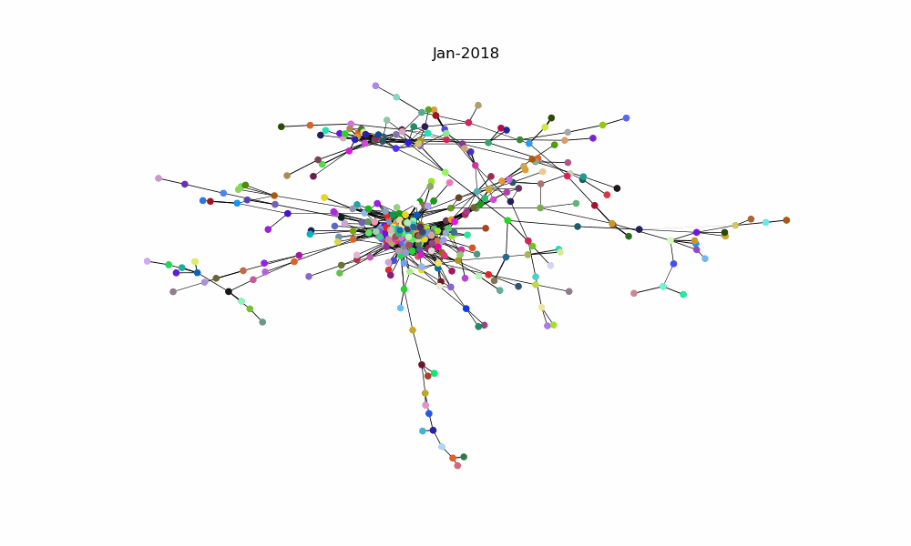
An example of a tool that has been previously discussed in Fasanara’s ‘’Thematic Research | Measuring Systemic Risks’’ is the Market Structure System Resilience Indicator (SRI). This tool allows to quantitatively asses the fragility of the market based on its network structure. Additionally, one can plot the network for visual analysis (and some pleasant eye-candy). Below there is an example of this tool in action. In particular, the GIF shows the week-by-week dynamics of the network structure of stocks in the S&P500 since January 2018.
ETAS Early Warning System
5-Day Crash Indicator
Carlos Saenz de Pipaon
Fasanara Analytics
The modelling framework of this new study is based on the Epidemic-Type Aftershock Sequence model (ETAS) developed by Ogata in 1988, which has been widely studied by geophysicists over the years. It models the occurrence rate of earthquakes (seismic activity above a given threshold) as a Hawkes process. The methodology presented is a novel approach to market crash warning systems that proves to be effective and provides advantages over the VIX and other GARCH-based indicators. When used in conjunction with the existing Ricci Curvature-based indicators in Fasanara's toolkit it provides a powerful tool to alert of forthcoming turbulent markets.
Happy reading!
1 Introduction
The development and implementation of Early Warning Systems (EWS) for the prediction of financial crashes is of paramount importance for both practitioners and regulators. A large part of the literature regarding EWSs has been devoted to improving the models based on measures such as Value-at-Risk and Expected Shortfall. In this study we present an alternative approach to the development of an EWS that takes inspiration from the geophysics literature, more specifically earthquake prediction.
Large financial crashes are outliers with respect to the frequency distribution of price drawdowns which have special characteristics that may be exploited for their prediction. In the models developed below, price movements and seismic activity are treated as the same phenomenon in order to study and exploit their self-reinforcing. This allows the development of a family of models that, ultimately, allow the researcher to predict the probability of occurrence of a price movement above a chosen threshold in a given period of time. This framework provides highly insightful medium-term forecasts without imposing stringent assumptions on the tail-behaviour of error distributions.
In this paper, after describing the methodology involved in the ETAS family of models presented in [1], we review the results obtained from the implementation of a specific ETAS model. We then comment on how this fits along with the Ricci Curvature-based indicator already in Fasanara’s systemic-risk indicator toolkit. Finally we compare the ETAS indicator with the VIX and comment on some of the advantages the former has over the latter in our use-case.
2 Methods
The modelling framework of this study is based on the Epidemic-Type Aftershock Sequence model (ETAS) developed by Ogata in 1988 [6], which has been widely studied by geophysicists over the years. This models the occurrence rate of earthquakes (seismic activity above a given threshold) as a Hawkes process [4]. The Hawkes process is a mutually self-exciting temporal point process, intuitively this means that occurrence of past points (crashes in the case under study) makes the occurrence of future points more probable.
Consider a event process (t1, m1), . . . ,(tn, mn), where ti defines the time and mi defines the mark of the event. Let Ht = {(ti , mi) : ti < tg} represent the entire history of events up to time t. Then the conditional intensity of jump arrivals following a Hawkes process is given by

where µ ≥ 0 and g (s − ti , mi) > 0 when s > 0 and 0 elsewhere. This conditional intensity can be broken down into its two components: (i) the constant term µ, and (ii) the self-exciting triggering function, g(s). The latter, g(s) is a function which depends on the time intervals between the occurrence of previous jumps at times ti and time t, as well as the size, mi , of these jumps. Notice that in the case relevant to us, events are negative price jumps whose magnitude is larger than a given threshold, i.e. market crashes.
Event-triggering functions, g(s)
In this study we consider two event-triggering functions, g(s), these are

where K0 is a parameter which controls the maximum intensity of event triggering for both functions. In addition, for Equation 3, K0 also controls the expected number of events triggered by an event. Similarly, this amount which we call the direct descendants of an event, is controlled by γ in Equation 2. The function c(mi) controls the influence that the size, mi , of past events has on the intensity with which future events are triggered.
For each of the two triggering functions above the probability of an event triggering decays over time. As the subscripts suggest, for Equation 2, probability decays according to a powerlaw distribution while for Equation 3 it decays according to an exponential distribution. The rate at which this probability decays is controlled by parameters ω and β, respectively. As these parameters become larger, the rate of decay of the triggering probability becomes faster.
Distribution of the sizes of excess magnitude events, G(χ)
As shown in the literature [5], the sizes of excess magnitude events with respect to a given chosen threshold (usually a given percentile in the distribution of all events) follow a Generalized Pareto Distribution defined by

where...
In this study we analyse models with both η = 0 and η 6= 0. In the first case, when the scale parameter η = 0, the hypothesis is that the sizes of future triggered events are unpredictable. Conversely, when the scale parameter is history-dependent, η 6= 0, the hypothesis is that the size of future events depends on the times and sizes of past 2 events and therefore these help to predict the former. As η increases, the influence of past events on future events increases. Furthermore, the mean and variance of the distribution Gξ,σ(t)(χ) of the sizes of excess magnitude events scales with σ(t). This means that as φ or η increase, the sizes of events modelled tend to be larger (higher mean size) and deviate more from the mean size.
Impact functions, c(mi)
The choice of an exponential function as the impact function, c(mi) is widespread in the geophysics as well as the finance literature. In our framework, we study this as well as other impact functions should not be explored and compared. The three functions to be implemented are:

The Pareto function as an impact function was introduced by Grothe et al. in [2] and the argument for it’s use is that the percentile of magnitude of the event in the conditional distribution from which it is drawn is valuable information that should be considered. Note that Gξ,σ(t) (mi) is again the Generalized Pareto Distribution of the sizes of excess magnitude events defined in Equation 4, mi is the magnitude of event i and M0 is the minimum magnitude of an event. Here α controls how the size of an event affects the probability of triggering other events. When α > 0, the probability of triggering events increases with the size past events (mi). When η > 0 the size of events is expected to be more extreme when the tension in the financial market is high. Using Equation 7 as the impact function when η > 0 the impact of extreme events in turbulent periods is smaller than in tranquil periods, when the probability of having these events is lower.
The full model
Putting all together, there are three main choices that can be made in order to build a complete model for the conditional intensity of jump arrivals λ (t|θ; Ht). These are:
1. the triggering function, g(s), the general function that defines how the times and magnitudes of previous events influence future events
2. the binary scale parameter, η, which controls if g(s) has any impact on λ (t|θ; Ht)
3. the impact function c(mi), which controls of the influence of the magnitude of an event on the triggering intensity of future events.
Different combinations of the three items above allow for 16 different models within this family of ETAS models that can be tested and compared. The way to do so is to estimate the parameters θ = {µ, K0, γ, ω, β, α, ξ, φ, η} for each of the models and then backtest these models on unseen data by the model in order to prevent any ”look-ahead” bias. The estimation of the parameters of the model, θ, can be done using Maximum Likelihood Estimation. The log-likelihood function maximised is given by
In our case, we used the Nedler-Mead algorithm to optimise this function. Being a numerical search algorithm, each time a model is calibrated, the maximisation was repeated 100 times in order to ensure the output is the global optimum and not a local optimum.
After obtaining estimates for the parameters of the model, one can calculate the probability of occurrence of an event following a Hawkes process with conditional intensity λ (t|θ; Ht) between times tn−1 and tn. This is given by


This probability forms the basis for the Early Warning System that can be implemented in order to signal potential future market crashes days in advance.
3 Early Warning System Calibration and Results
In this section, we present the results of the implementation of one of the variations of the model. In particular, we use the exponential event-triggering function (3) and the power-law impact function (6). The data used for the entire calibration process was the closing price of the S&P500 between January 2nd 1957 and September 1st 2008. We refer to this time period and data as the calibration period/data.
We then tested for the prediction of daily crashes of different sizes, namely those greater in magnitude than the 95%, 97% and 99% of total crashes, between January 2 2010 and January 21st 2020. For the data used, these correspond to daily moves of -1.97%, -2.36% and -3.24% respectively. This choice of this time period, which we call the validation dates, prevents any look-ahead bias in the model as the calibration period is before it without any overlap between the two.
Figure 1 shows the output of the model for the >97% case. For the validations dates, the top 3% largest drawdowns correspond to a total of 193 daily crashes, for which the ETAS model correctly detected 128, giving a hit-rate of 66% when using a 10% threshold as an alarm for a crash in the following five days, this proportion is displayed in Figure 2. This 10% threshold was chosen as the best balance between prediction power and false-signal rate out of the 8 different thresholds tested as given by Hanssen-Kuiper Forecast Skill Score [3]. Note that the choice of this threshold could be optimised further but this may lead to over-fitting of the model, something we surely want to avoid.


Figure 2: Graphical representation of the crash-signalling hit-rate of the ETAS model implemented when using a 10% crash probability threshold.
3.1 Merging with Ricci Curvature-based market fragility indicator
As a continuation to previous research done at Fasanara, we now compound the results of the ETAS 5-day crash indicator to the results of the Ricci Curvature-based (RCB) indicator [7], already in Fasanara’s toolkit. This indicator is by representing the market as a network of stocks that can be derived from the correlations among them. The RCB indicator is correlated with market fragility, or systemic risk, and signals times when there is a spike in this fragility. Figure 3 shows the evolution of the RCB indicator for the S&P500 over time.


Figure 3: S&P500 daily closing price between 2000 and 2020 overlaid with Ricci Curvature-based indicator.
The merging of the ETAS and RCB indicators therefore signals periods of time where: (i) there is a high probability of a large daily crash can occur, and (ii) when the market is in a particularly fragile state. In Figure 4, we display the times these two indicators signal their respective outputs. The threshold chosen here for the ETAS models is less conservative, giving a signal when the probability of a >97% percentile negative movement is >20%.
This figure shows that, previous to the most turbulent market movements, both indicators signal a high probability of a crash and a high market fragility. This is especially evident during the marked times where there is a clustering of signals for both indicators as well as many periods of overlap between these two signals. It is during these overlaps or frequent alternation of signals that investors have to be particularly careful and observant of the developments of the market.
Figure 1: Daily closing price for the S&P500 between 2010-2020 (in black) along with probability of daily crash in the top 3%-percentile during the following 5 days given by the ETAS model (in red). Strongest signals are marked with a red triangle

More Cookies


